|
Table of Contents | Go to the Japanese version of this page. |
| |
| |
Welcome to the help page for the Java-Powered Simulation for Structural Vibration and Control. This program allows you to compare the effect of using two different control systems to reduce the structural response of an "uncontrolled" structure subjected to earthquake excitation. The two control systems, chosen because of the widespread interest in this class of systems (Soong 1990; Housner et al., 1994; Fujino et al. 1996), are the tuned mass damper (TMD) and the hybrid mass damper (HMD). Note that such controllers can be experimentally verified using the benchscale AMD experiment manufactured by Quanser Consulting, Inc.
This program allows you to vary the control system properties and control objectives and to perform "what if" studies so as to better understand the control design process. The program can calculate and animate the structural responses under the El Centro, Hachinohe, Northridge and Kobe earthquakes, as well as determine the transfer functions of the uncontrolled and controlled systems. Three cases can be considered:
The TMD/HMD mass is rigidly attached to the structure.
The TMD/HMD mass is attached to the structure by a spring and damper.
In addition to spring and damper employed in the previous case, a control actuator is installed between the TMD/HMD mass and the structure. Note that this version of the program does not include actuator dynamics (Dyke, et al. 1995). Future versions of the program will include this enhancement.
![[picture of java page]](help.gif)
Structure Mass:
The mass of the structure. The default value is
![]() tons.
tons.
Structure Natural Frequency:
The natural frequency of the structure. The default value is
![]() Hz.
Hz.
Structure Damping Ratio:
The damping ratio of the structure. The default value is
![]() .
.
TMD/HMD Mass Ratio:
The ratio between the TMD/HMD mass and structure mass. The default
value is ![]() .
.
TMD/HMD Natural Frequency:
The natural frequency of the TMD/HMD. The default value is
![]() Hz.
Hz.
TMD/HMD Damping Ratio:
The damping ratio of the TMD/HMD. The default value is
![]() .
.
An LQR controller is calculated based on a quadratic performance index (see Technical Background) that weights the structural responses. The parameters q1-q4 weight the following responses:
q1 - structural displacement.The weighting on the control action is taken to be unity.
q2 - HMD displacement.
q3 - structural velocity.
q4 - HMD velocity.
Check the radio buttons to indicate which responses you wish to display.
Width of the excitation/response windows (in seconds) used during the animation. If your computer can't display the animation smoothly, please make this number smaller.
Scale used for the motion of the ground in the animation. The ground motion may not be very noticeable in the animation when the same scale is used for both the structural response and the ground motion. The ground displacements are multiplied by the value in this box before they are displayed in the animation. This scale factor does not affect the response calculations nor does it affect the animation when the Relative Motion option is selected in the Animation Frame. An upper limit is set on the value so as to keep the animation within the window boundaries. The default value is 1.
Calculate: Redo the calculation according to the current input parameters. When you change the structure parameters, TMD/HMD parameters or LQR control weights, you must hit this button to recalculate the responses and bode plots. Since the integral step 0.02 sec (50 Hz) is used during the earthquake response calculation, the structure natural frequency and TMD/HMD natural frequency should be less than 10 Hz to obtain an accurate result.
Animate: Animate the structural motion under the earthquake excitation. After the animation begins, this button will change to the "Stop Animate" button. Hitting this button again will stop the animation.
Reset Parameters: Reset the parameters to default values.
Help: Hitting this button will bring you to this help page.
The animation frame shows the structural system as it undergoes the earthquake excitation. Each of the three cases mentioned above can be animated by appropriate selection in the left menu associated with this frame. Also, you can choose to animate absolute or relative motion of the structure. Absolute Motion displays the response of the structure from an inertial reference frame. Thus, the motion of the ground is seen here. Relative Motion shows the response of the structure from a reference frame attached to the base of the structure.
The earthquake signal frame shows the current earthquake signal you are now using. There are four earthquake signals you can use:
El Centro earthquake signal: North-south component recorded at Imperial Valley Irrigation District substation in El Centro, California, during the Imperial Valley, California earthquake of May 18, 1940. The magnitude is 7.1 and the maximum ground acceleration is 0.3495g.
Tokachi-oki (Hachinohe) earthquake signal: North-south component recorded at Hachinohe City during the Tokachi-oki earthquake of May 16, 1968. The magnitude is 7.9 and the maximum ground acceleration is 0.2294g.
Northridge earthquake signal: North-south component recorded at Sylmar County Hospital parking lot in Sylmar, California, during the Northridge, California earthquake of Jan. 17, 1994. The magnitude is 6.8 and the maximu ground acceleration is 0.8428g.
Hyogo-ken Nanbu (Kobe) earthquake signal: North-south component recorded at Kobe Japanese Meteorological Agency (JMA) station during the Hyogo-ken Nanbu (Kobe) earthquake of Jan. 17, 1995. The magnitude is 7.2 and the maximum ground acceleration is 0.8337g.
You can choose to display the displacement or the acceleration corresponding to each earthquake signal. The strong motion data used in the Java program can be download from here.
The bode plot frame can display the magnitude plot and phase plot for the transfer function from ground acceleration to structural displacement, structural velocity, structural acceleration, TMD/HMD displacement, TMD/HMD velocity, TMD/HMD acceleration or control actuator force. The particular transfer function displayed corresponds to the response shown in the Time Response Frame.
The time response frame displays the system's response due to the earthquake signal shown in the Earthquake Signal Frame. It can show the structural displacement, structural velocity, absolute structural acceleration, TMD/HMD displacement, TMD/HMD velocity, absolute TMD/HMD acceleration or control actuator force. Peak response information is displayed in the lower portion of this frame.
The structure stiffness
![]() ,
structure damping
,
structure damping
![]() ,
TMD/HMD stiffness
,
TMD/HMD stiffness
![]() and TMD/HMD damping
and TMD/HMD damping
![]() can be calculated as following,
can be calculated as following,
where,
is the structural displacement relative to the ground (m).
is the structural velocity relative to the ground (m/s).
is the structural acceleration relative to the ground (m/s2).
is the ground acceleration (m/s2).
where,

is the TMD/HMD displacement relative to the ground (m).
is the TMD/HMD velocity relative to the ground (m/s).
is the TMD/HMD acceleration relative to the ground (m/s2).
The state-space model is:
is the applied actuator force (N).
is the actuator driven signal (V).
is a constant gain of the actuator (N/V).
is arbitrarily chosen in the program as
.
or
or
![z = [x_1 x_2 (dx_1/dt) (dx_2/dt)]'](image126.gif)
![y = [x_1 x_2-x_1 (dx_1/dt) (dx_2/dt-dx_1/dt) (d^2x_1a/dt^2) (d^2x_2a/dt^2)]'](image127.gif)
is the absolute acceleration of the structure (m/s2).
is the absolute acceleration of the TMD/HMD (m/s2).
For the control design, state feedback with noiseless measurements is assumed. By using the LQR optimal algorithm, the optimal gain matrix K is calculated such that the actuator driven signal
minimizes the quadratic cost function
![J = 0.5 * int(z'*[Q]*z+u^2,t=0..infinity)](image131.gif)
for the continuous-time state-space model given above where Q is the state weighting matrix with the form:
![[Q] = diag([q_1 q_2 q_3 q_4])](image132.gif)
Recall that the weighting on the control signal is unity. Here the ground acceleration is treated as an external disturbance for the HMD system.
The optimal gain matrix K is derived from S by
, which is the solution of the associated Algebraic Riccati Equation
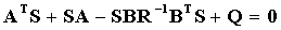
Algorithms for the solution of the Algebraic Riccati Equation are thoroughly discussed in Arnold and Laub (1984).
Closing the feedback loop with an optimal gain matrix K, the system model has the following form:
![(dz/dt) = [A-BK]*z + [E]*(d^2x_g/dt^2)](image133.gif)
Although the actuator dynamics are not accounted for in the analysis, the role of actuator dynamics and control-structure interaction is important to the design of the protective systems such as the HMD system (Dyke et al., 1995). Future versions of the program will include these phenomena, as well as allow for investigation of output feedback methods.
![[structure picture]](bamd.jpg)
Experimental verification of structural control strategies is essential for eventual full-scale implementation (Dyke et al., 1996a,b). However, few researchers have facilities readily available to them that are capable of even small-scale structural control experiments. Recently, a bench-scale structural model of a building with an active mass driver has been developed that portrays the salient aspects of full-scale structural control implementations, including: control-structure interaction, actuator and sensor dynamics, actuator saturation effects, limited availability of sensors, output feedback design and digital control implementation (Battaini et al., 1998). This active control experiment, designed and manufatured by Quanser Consulting, Inc., has been shown to be an effective tool for education and for familiarizing practitioners with control system design and the associated challenges. |
The support of the National Science Foundation under Grant No. CMS 95-28083 (Dr. S.C. Liu, program director) is gratefully acknowledged. In addition, we would like to thank Prof. Yozo Fujino of the University of Tokyo for his help in securing the Kobe and Hachinohe earthquake records.
Arnold W.F., III and Laub A.J. (1984). "Generalized Eigenproblem Algorithms and Software for Algebraic Riccati Equations," Proc. IEEE, 72, pp. 1746-1754.
Battaini, M., Yang, G., Spencer Jr., B.F. (1998). "Bench-Scale Experiment for Structural Control," Journal of Engineering Mechanics, ASCE, in press.
Dyke S.J., Spencer Jr. B.F., Quast P. and Sain M.K. (1995). "The Role of Control Structure Interaction in Protective System Design," Journal of Engineering Mechanics, ASCE, Vol. 121, No. 2, pp. 322-338.
Dyke, S.J., Spencer Jr., Quast P., Kaspari Jr., D.C. and Sain, M.K. (1996a). "Implementation of an Active Mass Driver Using Acceleration Feedback Control," Microcomputers in Civil Engineering: Special Issue on Active and Hybrid Structural Control, Vol. 11, pp. 305-323.
Dyke, S.J., Spencer Jr., B.F., Quast, P., Sain M.K., Kaspari Jr., D.C. and Soong, T.T. (1996b). "Acceleration Feedback Control of MDOF Structures," Journal of Engineering Mechanics, ASCE, Vol. 122, No. 9, pp. 907-918.
Fujino, Y., Soong, T.T. and Spencer Jr., B.F. (1996). "Structural Control: Basic Concepts and Applications," Proceedings of the ASCE Structures Congress XIV, Chicago, Illinois, pp. 1277-1287.
Housner, G.W., Masri, S.F. and Chassiakos, A.G., Eds. (1994). "Proceedings of the 1st World Conf. on Structural Control," Pasadena, CA..
Soong, T.T. (1990). "Active Structural Control, Theory and Practice," Longman Scientific and Technical, Essex, England.
![[state derivative equations]](image123.gif)
![[sensor equations]](image75.gif)